Analyzing the correlation between hitting performance and salary for MLB athletes using machine learning models and using this correlation to predict future data.

• Jupyter Notebook
• Python
• Pandas
• Flask
• Psycopg2
• SQL
• PgAdmin4
• Tableau
• Final Project Dashboard (Tableau)
• Project Presentation
• Project Dashboard (Google Slides)
• Data: batting.csv, batting_filtered.csv, batting_salary.csv, salary.csv, salary_filtered.csv

The SQL Files folder contains all the necessary scripts to create, filter and merge the databases used in this project.

This folder contains 3 main files:

• The document that contains the schema of the two main tables used in the database(batting.csv and salary.csv) is schema.sql
• The document that contains the filtering of these two tables from 2009 to 2014 is filtering.sql
• The document that merges both filtered datasets is merge_views.sql

• Our project revolves around the topic of salaries in Major League Baseball(MLB) from 2009 to 2015 and the relationship that batting stats have in regards to a player's salary. We are going to look at the hitting stats for the years 2009-2014 to gain insights on both the hitting and salary stats. Once we have completed our extraction and transformation of the data, we will then test the 2015 data in a linear regression model to see how much of a correlation hitting performance has with the salary a player is paid. It is our hypothesis that there will be a very strong correlation between these two variables.

• We chose this topic because we all shared an interest in both sports and finance and one question that utilized both of these interests was the salary of athletes. We then narrowed that initial interest down to the sport of Baseball and specifically hitters because unlike their pitching counterparts, hitters play far more frequently and are almost always the highest paid players on the team. In order to complete this project our first order of business was simply to look at our dataset, which gave us salaries from 1985-2015. To narrow our scope and for the sake of relevance, we decided to focus on a 5 year period of 2009-2014 as our training data and the singular year of 2015 as our testing data. This would allow us enough information we believe to analyze the data and test our hypothesis.

• Based on the hitting performance of a player, is there a strong correlation between hitting performance and how much they are paid?
• Is it possible to predict the salary of a player using a linear regression model with the data given?
• Given a players salary for 2015, was this player overpaid or underpaid?
• What teams were the most successful at avoiding overpaying players, and who had the most players who were overpaid?

• We pulled our Data from the Lahman's Baseball Datasets on SeanLahman.com. This website has baseball data from 1871-2021. This information had the hitting statistics we are using from 2009-2015 and the salary data from 2009-2015 as well. The hitting dataset had 22 columns and the salary dataset had 5 columns. They both shared two IDs which we could choose to merge on, and we chose to use the player_id column as they held unique IDs for each player in the dataset.

After merging our two tables (Batting and Salary), we decided to filter them using views and merge this filtered data. The created views can be seen below.

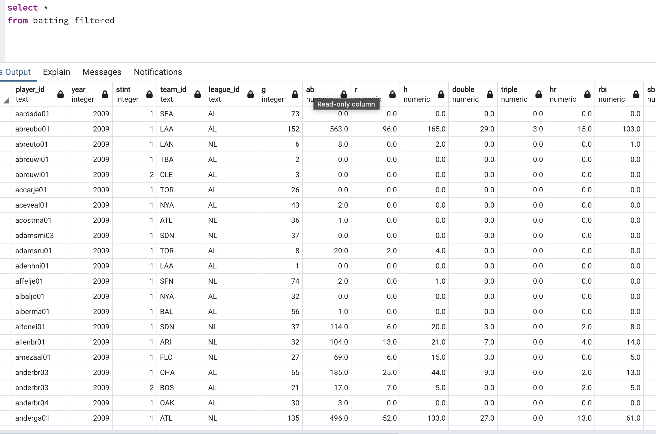
Batting filtered and Salary filtered contain the filtered data from 2009 to 2014. The batting_salary view contains the merged views. In the image below, we can see how the data looks like after the merging process.

These are the base metrics we obtained from Kaggle. These metrics do not require any calculation, however, these are the base for our analysis.

• 'year',
• 'g' - games played in the season
• 'ab'- at-bats in the season
• 'r' - runs scored in the season
• 'h' - hits in the season
• 'double'
• 'triple',
• 'hr' - home runs in the season
• 'rbi' - runs batted in during the season,
• 'sb' - stolen bases
• 'cs' - caught stealing
• 'bb' - walks in the season
• 'so' - strikeouts in the season
• 'ibb' - intentional walks in the season
• 'hbp' - hit by pitches in the season
• 'sh' - sacrifice hits
• 'sf' - sacrifice flies
• 'g_idp' - grounded into double play
• 'single'

• 'slg %' - slugging percentage, Slugging percentage represents the total number of bases a player records per at-bat
  • 
• 'obp' - on base percentage, OBP refers to how frequently a batter reaches base per plate appearance
  • 
• 'batting avg' - batting average is determined by dividing a player's hits by his total at-bats
  • 
• 'tb' - total bases, refer to the number of bases gained by a batter through his hits
• 'ops' - On-base plus slugging is a sabermetric baseball statistic calculated as the sum of a player's on-base percentage and slugging percentage
  • obp*slg %
• 'rc' - runs created estimates a player's offensive contribution in terms of total runs
• 'babip' - batting average on balls in play measures how many of a batter’s balls in play go for hits
• 'pa' - plate appearance (denoted by PA) each time a player completes a turn batting
• extra base hits (xbh) as the model seemed to find more information in power categories
• isolated power (iso) which is another power stat that we hoped would give our model more clarity.
• walks per plate appearance (bb/pa) and strikeouts per plate appearance (so/pa)

• The first step in our Machine Learning phase was preprocessing and to check to see if any data was missing. Our dataset had no missing values, but once we started to engineer new stats, there were cases where a number was divided by 0 thus creating NaNs and so we filled those with zeroes. Then we decided to bin the years (even though they were viewed as integers) into groups of 0,1,2, etc. We considered normalizing the data, but decided against it as our model standardizes the data prior to testing.

• The feature engineering process involved creating additional columns based on the data that was given as well as giving more information to our dataset. The first step was to create more columns that sufficiently utilized the full extent of the stats present.

• While our set had a hit column, this column did not show how many of those hits were singles. Additionally, our dataset did not combine all of a player's plate appearances (as at-bats leaves out any non-contact event, walks, sacrifices). Therefore, we created a column that encapsulated these aspects of our data.

• In the world of baseball there has been a growth in certain stats that have proven to be a strong indicator of a batter's value. These stats were also created and added to the dataset

  • slg %
  • obp
  • batting avg
  • tb
  • ops
  • rc
  • babip

• We created several heatmaps to look at correlation in order to evaluate our dataset further. Subsequently, a question was posed, "Could we gather any information from the team_ids in relation to salary?". Therefore, after creating both a new dataset and a heatmap, we found some teams (such as NYA and PHI) did have a small positive correlation. After using the get_dummies function of pandas we chose to include these columns as well.

• The reason for adding additional stats is that our dataset has a significant number of players (25%) who have 1 or less at-bat, and so by adding additional features we hoped that the ML model could perceive and identify the values more clearly with this additional information.

• The data was initially split into the standard 75-25% split that skllearn defaults to. We used the salary feature as the one for testing. After running additional tests and playing with the information, we decided to adjust that to 80-20% as it increased our testing % to 18.6% from 17.3%.

• We chose a linear regression model as we had a very clear relationship we wanted to look at with hitting stats and their relationship to salary. If we could provide hitting statistics as our independent variable, how would that affect our dependent variable of salary? We were able to gather this information and with the simplistic nature of implementing a linear regression model we moved forward with this as our Machine Learning Model.

  • Pros of linear regression models

    • The benefit of using the linear regression model is primarily in its simplicity. It is very easy to implement and interpret the relationship beyween our chosen variables.
    • The simplistic nature of a linear regression model makes it very friendly from a computional aspect as it is able to run large amount of data in a very quick and efficient manner.
    • Linear regression is prone to over-fitting, but it can be fixed using reduction techniques.

  • Cons of linear regression models

    • The foremost issue with using this model is that it assumes there is a straight-line relationship between the independent and dependent variables and in real life instances this is rarely the case.

    • They are greatly affected by outliers. For example, in our model intentional walks, "ibb" had a number of outliers and when removed it greatly reduced our model's accuracy. The model one way or another is swayed by these powerful outliers.

    • Optimization can prove to be very time consuming and there is a risk of overfitting the model. In using the reduction features to combat overfitting, you will risk overfitting irrevelant features and this could be both time-consuming and point your data in the wrong direction.

• Our original linear regression model struggled to find a correlation between hitting statistics and the salary of hitters. This could be due to there being a number of additional extraneous factors that affect pay for a hitter. This led our team to reevaluate our analysis of our data and we concurred that we could classify players on whether they would be considered "Unpaid" or "Overpaid".

• The first thing we did was determine how to set the parameter that would serve as the measurement for how we would test this statement. We knew we wanted to use salary, but after looking at our data it was very skewed to the left. Consequently, for each season we took the median instead of the mean. This is the preferred choice with skewed datasets such as ours.

• Then we created two new columns. After getting the median amount for each year, each player was classified as either "highly paid" or "under paid". This would be the question our model would try to answer, "Can we classify correctly, if a player was "highly paid" or "under paid" from the hitting statistics?".

• We kept our original Data and created stats, we also added

  • Extra base hits (xbh) as the model seemed to find more information in power categories
  • Isolated power (iso) which is another power stat that we hoped would give our model more clarity.
  • Walks per plate appearance (bb/pa) and strikeouts per plate appearance (so/pa)

• We also removed anyone who did not have an at-bat in our dataset. This amounted to about 20% of our data. This allowed us to remove almost all pitchers and would leave only those who hit on an infrequent basis.

• Our original model used StandardScaler, but MinMaxScaler is supposed to handle datasets with a larger number of outliers, which is more in line with our dataset.

• We chose a classification model and specifically Logistic Regression as we wanted to answer the question of whether our model could classify someone as over or under the median. The simplistic nature and application of a Logistic Regression Model led us to go towards this direction. We felt that our data would struggle to find a way to pinpoint a numerical prediction, but the data could answer classification questions better.

  • Pros of logistic regression models

    • The most beneficial aspect of this model, similarly to its Linear counterpart, is its simplicity. This means it needs less computing power, and due to this it can be often a model to initially measure performance.

    • The model allows for the importance of features to be viewed. We can see how important a feature might be or if it lacks a connection with the question.

    • Classification is used quite often with these types of model and it can be used effectively in singular class as well as with multi-class classification when needed.

  • Cons of logistic regression models

    • Non-linear problems can't be solved with logistic regression due to its linear nature, and this often leads to engineering more features and transforming the data to answer the questions someone might pose.

    • Logistic regressions requires a large dataset and also an ample amount of training examples for it to succeed in classification.

    • Due to the simplistic nature of the model, it struggles with complex relationships. This model can be outperformed quite easily by Neural Networks if you are willing to invest the time and capital to create one.

• As stated earlier we chose to use MinMaxScaler as this package deals with data that has a larger amount of outliers.

• We removed the salary column, and we also removed the columns stating if a player was highly paid or under paid.

• The training and testing was split into a 75/25 split after multiple attempts to see how this affected the results.

• In our Logistic Regression model we had

  • True Positive (TP) = 344
  • False Positive (FP) = 202
  • True Negative (TN) = 277
  • False Negative (FN) = 107

• This led to an accuracy of the binary classification of 66.7%.

• We looked into other classification models and they produced the below results.

• Tableau Dashboard

Interactive Feature: You can select which year or years you'd like to view the data for.

Interactive Feature: You can select which year or years you'd like to view the data for.

Interactive Feature: You can select which year or years you'd like to view and you can select which stat you'd want to see the correlation against salary for.

• The first recommendation we noted that we would have looked at if we had more time was removing pitchers from the dataset. The ability of pitchers to hit created situations where high salary players that were earned due to pitching cause confusion for our model.

• Another recommendation would be to create a model that would be able to predict salaries and classifications that would take variables from the hitting statistics that were strong and combine it with pitching statistics, fielding statistics, general information (such as age, team, contract status), and take the variables that were strong in each category to create a better model.

• Further working on how to effectively use or remove outliers in our dataset to help train the model. We had situations where certain statistics were 30 times over the standard deviation, but it hurt our accuracy when they were removed.

• Could it be possible to keep player IDs in the dataset and would that have helped with model accuracy? If the model could have known that a particular player who was paid a high salary previously, was just hurt for this season and that created a large difference in stats, they could have been able to know this is still a high paid player.

• We could look to see how a deep learning model would have performed on the dataset versus the simplicity of regression.

• Would it have been easier to choose pitching statistics? There would have been very few outcomes that a batter would have shown up in the dataset, as opposed to a pitcher showing up in the hitting dataset.

• The years we chose to test. We had salary data from 1985, if we chose an early time period would that have changed our results?

• The classification model gave much greater results than our prediction model, if we had known that we would have found more success with this outcome, we could have started with this question and this would have given us more time to refine and adjust the model.